Comparing Performance of Different Production Management Approaches

Abstract: This paper summarizes the key differences between: Traditional Batch, Traditional, Cell, Just-In-Time, Lean, Theory of Constraints and Agile production control methods. A production simulation model compares common measures (Work-In-Process, Flow Time, Efficiency, Throughput, Profit and Return on Investment) for each of the control methods.

Background: Every manufacturing company is on the road to improvement. While most companies are going the right way on the road, many are unhappy with their slow rate of improvement. As a result, nearly every company is asking serious questions about their processes. "What should we change to next?" This paper attempts to help the reader understand several alternative control methods and compares the different methods on equal ground.

There are just about as many methods for implementing a manufacturing control strategy as their are manufacturing firms. So, for this paper, each control method will be presented in its simple and straightforward application.

The Challenge

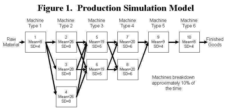
Lets consider a typical production process of 10 available machines of 6 different types. Raw materials enter from the left and flow through the production process towards the right where the products become finished goods. Figure 1 shows how each product flows through one of each of the six types of machines. In this linear flow process, there are no assemblies or disassembly processes. Where multiple machines are available of a common type, the product may flow through any one of those machines without a set-up.

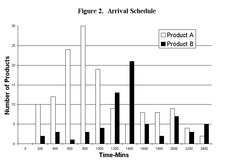
There are two different products . Product A accounts for 2/3rds of the workload and Product B accounts for 1/3rd of the workload. The raw materials arrive according to a weekly schedule. Exactly 120 Product A parts and 90 Product B parts arrive one at a time over 5 each 8 hour shifts (2400 Minutes). The same schedule repeats each week. Figure 2 is a histogram that shows the relative intensity of the arrivals by product over the week.

To add reality to this model, each machine work speed varies according to a normal distribution. The mean (estimated value) and standard deviation (measure of variance) is noted in Figure 1. In addition, each machine is subject to random breakdowns. Breakdowns occur every 100 minutes on the average (drawn from a negative exponential distribution) and last about 10 minutes (also drawn from a negative exponential distribution). This means the machines are only available 90% of the time.

Theoretically, this system should be able to produce 216 parts per week. The limiting process is Machine Type 4 which has two machines (7 and 8) processing with a mean of 20 minutes. Machines 7 and 8 produce two parts every 20 minutes or average 10 minutes per part. This is 240 parts per week. These machines operate 90% of the time so the theoretical maximum is 216 parts per week. These simulation models runs for 2 1/2 weeks (100 hours).

Production Process Control Options:

Traditional Batch Production: In traditional batch production, raw material is grouped together in a batch and the batch is routed to the machines and processed at the machines as a batch. Each part is processed separately but each part waits for the others to be processed and then the batch moves as a whole to the next process. In this model, machine efficiency is emphasized and work flow time is not. This method is common where material handling is a problem. A batch could be a 24 disk cassette, a 120 piece flat pallet or 1000 punched parts in a bin. In the batch simulation model, the batch size is 10. Ten parts all travel together through each process.

Traditional Production: The traditional production model is a push system with a batch size of one. In this model, raw material enters the production process as soon as it is available. When work on one machine is completed, the product moves automatically to the next production process and chooses the machine with the shortest queue. The traditional model pushes raw material down the production line in an effort to run at maximum efficiency. In the simulation model, work is processed first-in-first-out which guarantees that products will come out sooner or later. This may not be the case in the real world where priority work exists.

Traditional Cell Production: One technique to help manage a complex manufacturing system is to divide the shared resources into work cells that can be more effectively managed. In this manner a cell of equipment is dedicated to producing one category of product and is not available for other work. In the simulation model, Product A is routed through machines 1->2 or 3->5->7->9->10. Product B is routed through machines 1->4->6->8->9->10. The constraint for Product A is Machine 7 at 20 minutes each. The constraint for Product B is Machine 4 at 26 minutes each.

Just-In-Time: The Just-In-Time production control model is a pull system. Each work station only produces the quantity of products requested by the customer in subsequent operations. Work control often uses a Kanban card to control the flow of parts through the system. When a customer wants a product, the Kanban card is given to the previous process machine and that machine passes the requested product to the customer. The customer starts work on the product recieved and the previous process starts work on preparing the next product for the customer. In this simulation model, the demand is from right to left. As a machine on the right needs a product, machines on the left produce the product just in time. A Just-In-Time control process is characterized by low Work-In-Process inventories situated throughout the plant between each machine. Two Just-In-Time simulations are shown here. JIT Kanban of 1 allows 1 product of Work-In-Process between each machine. JIT Kanban of 3 allow 3 products of Work-In-Process between machines.

Lean Manufacturing: Lean manufacturing attempts to maintain low Work-In-Process inventories and avoid excess investments (excess capacity). Lean and be either a push or pull system. Work-In-Process is limited and excess capacity is trimed away. In this simulation, a push model is used with a maximum of 5 products between machines. And the work process times are slowed to an average of 10 minutes per product for each type of machine (machines 1, 9 and 10 are 10 minutes per product; machines 2, 3 and 4 are 30 minutes per product; machines 5 and 6 are 20 minutes per product). Standard deviations stayed the same.

Theory of Constraints: The Theory of Constraints work control process is based on three elements: The Drum (the speed or capacity of the slowest process), the Buffer (the amount of inventory allowed into the system before the constraint) and the Rope (the releasing mechanism for raw material). In the DBR process, every effort is made to increase the efficiency of the constraint even at the determent of other measures. The inventory level (the buffer) must insure the constraint never runs out of work. The rope mechanism restricts all inventory not needed to protect the constraint from entering the system. Each machine is directed to work as fast as it can when there is work and to sit idle if there is not work.

Agile Manufacturing: The concept of Agile manufacturing is flexibility. With agile processes the manufacturing line changes rapidly to changes in demand. If the product demand during one part of the week changes, the resources are realigned to meet the new demand. Agile manufacturing often includes multi-tasking of machines and multi-skilled operators. In this simulation, machine 1 is cross trained to help machines 2, 3 and 4. Machine 9 is cross trained to help machines 5 and 6. Machine 10 is cross trained to help machines 7 and 8. The cross trained machines only help the other machines when the queues build up on those machines and the cross trained machine is idle. In each case, the cross trained machine is not as quick as the machines it is helping.

Performance Measures

Several measurement factors are used to compare the results of these simulations.

WIP--Work-In-Progress. The simulation measures WIP as a rolling average. It uses an exponential smoothed average of WIP over time (alpha value of 0.02).

Flow Time--The Flow Time is the average of the actual flow time from when a product enters the production process until it is completed. Flow Time starts counting when the product raw materials are accepted.

Effc.%--Average Efficiency is a composite measure averaging the utilization of all ten machines.

Produce--The number of finished goods completed over the length of the simulation is reported. Each produced product is sold immediately.

Profit--Profit is measured as the number produced * (sales price - raw material price) less operating expenses. The sales price is $130 for each product. The raw material price is $50 per product. Operating costs are $300 per hour.

ROI--Return on Investment is a measure relating profit to the investment of the firm in fixed assets and in inventory. ROI is profit/(annualized capital charge plus inventory costs). The annualized capital charge for 100 hours is $50,000. Inventory is charged at raw material cost.

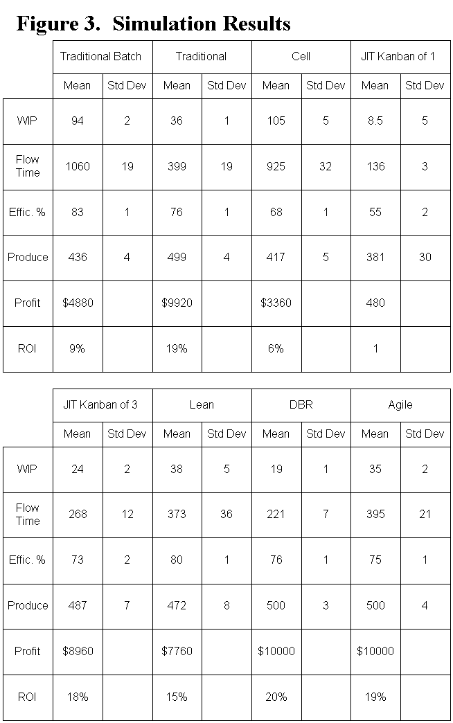
Each model was simulated 20 times for 100 hours. The performance measures are tabulated in Figure 3.

It is interesting to note the JIT Kanban 1 models had a very low WIP and the fastest flow time. And there was a very small standard deviation to the flow time prediction for this model. Unfortunately, it had the lowest production level.

Several models demonstrated high production capacity: Traditional, JIT Kanban 3, Lean, DBR and Agile. The models with the lower inventory and quickest response times were marginally better on their rate of return.

Low Work-In-Process levels and short flow times are desirable. It is also desirable to be able to predict delivery times (low variability in flow time). Having enough inventory to keep critical processes operating seems more important than keeping all machines at high levels of efficiency. Having flexibility to move resources around (as in the Agile model) is highly desirable.

Overall the DBR control mechanism provides high production levels, low flow times, accurate prediction of flow times and good cost figures.

About the Author: James R. Holt is an Associate Professor of Engineering Management at Washington State University-Vancouver. Dr. Holt teaches Operations Research, Simulation, Constraints Management, Organizational Management and Project Management. He is an Academic Associate with the Avraham Y. Goldratt Institute.